2.3. Verifying a Solution

In this section we shall explain a simple way to verify that you have computed correctly the shortest path between two nodes in a given graph, without having to rerun the entire algorithm. Suppose that the input is a directed graph \(G=(N,A)\), where each arc \((i,j) \in A\) (the \(\in\) symbol means “is an element of”) has a given length \(\ell (i,j) \ge 0\), and you wish to compute the shortest path from a given node \(s\) to each other node in the graph. In fact, you have run Dijkstra’s algorithm and computed that the shortest path from \(s\) to one node \(w\) consists of the the \(k+1\) arcs \((s,i_1), (i_1,i_2), \ldots, (i_{k-1},i_k), (i_k,w)\). You want to know some easy way to verify that you have computed the correct path, other than just running the algorithm again to see that you did each step correctly.

Consider the input in Figure 2.6. Can you give a convincing argument that you know that shortest path from node 1 to each other node? (Think about this before reading on!!)

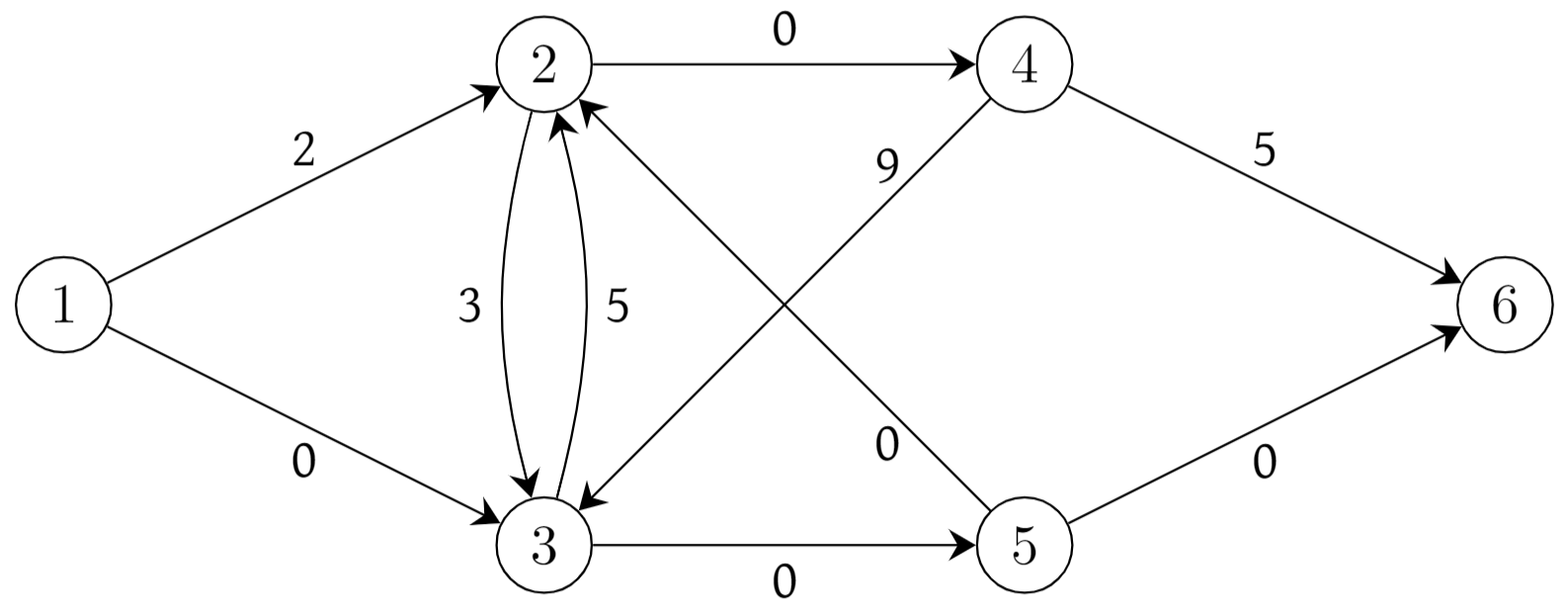
Fig. 2.6 An easy shortest path input

Since each arc length is nonnegative, then the length of any path is nonnegative. However, for each node \(i\) in Figure 2.6, it is quite easy to identify a path of total length 0 from the source to node \(i\). Since all path lengths are non-negative, then certainly a path of length 0 is a shortest path (because no path of negative length exists!) Of course, as in the example above, if the length of the whole path is 0, then the length of each arc in it must also be 0. (Because, once again, there are no negative length arcs.) This seems like a very special case, but the end conclusion will be that it is still a very useful and powerful idea.

The next step will be to consider a rather peculiar variant of the shortest path problem. In this new problem, we are given a graph as in the usual shortest path problem, plus each node \(i \in N\) has a special price \(p(i)\). In this new problem, we view the nodes as representing cities and the arcs as roads connecting them. When we travel along an arc \((i,j) \in A\), we incur a cost equal to its length \(\ell (i,j)\); in addition, whenever we enter a city we are given a present meant to entice us to stay in that city of value \(p(i)\). If we leave that city, we must pay that amount back. Once again, we return to our original input, as given in Figure 2.4, and add such \(p\) values, where each node’s value is specified in a box right next to it.

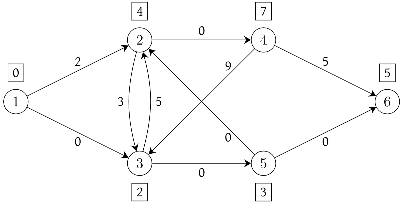
Fig. 2.7 A graph with node enticements

In general, what is the cost of our path from the source node \(s\) to node \(w\) (for our new problem)? Well, we must pay \(p(s)\) to leave the source, and we will get \(p(w)\) when we finally enter node \(w\). All of the other presents acquired en route must be paid back, so the total cost is

\[\ell (s,i_1) + \ell(i_1,i_2)+ \cdots+ \ell(i_{k-1},i_k) + \ell(i_k,w)+p(s)-p(w).\]

A shorthand notation for this is to write it as

\[\ell (s,i_1) + \sum_{j=2}^{k} \ell(i_{j-1},i_j) \ \ + \ell(i_k,w) + p(s)-p(w).\]

So we can think of the total cost of this path as its total length with respect to the original length function \(\ell\) plus \((p(s)-p(w))\). But this is true no matter which path from \(s\) to \(w\) we consider! Therefore, the cheapest path in this new setting is exactly the same as the shortest path for the original lengths. (Make sure you understand exactly why this is!) We have obtained an equivalent problem to solve; a path that is shortest for this new variant must be a shortest path in original sense, and vice versa. (Make sure you understand this; thinking about the specific example given in Figure 2.7 is probably helpful.)

Here is another view of the new problem, however. We would like to get rid of the fact that there are these two types of costs, arc lengths and “node enticements”, but still leave the problem unchanged, even in computing the cost of any path correctly. Here is a simple idea that might be seem a bit odd at first. Think about using an arc \((i,j)\). To use it, one must first leave node \(i\), then traverse arc \((i,j)\), and then enter node \(j\). All are required if we are to use arc \((i,j)\) at all. So the effective cost of traversing this arc is \(p(i)+\ell(i,j)-p(j)\). We define the adjusted length of an arc \((i,j)\) of the graph to be

\[\bar \ell (i,j) = \ell(i,j) +p(i)-p(j).\]

The total adjusted length of a path is the sum of the adjusted lengths of arcs in that path. It should be clear that the adjusted length of any path is exactly the quantity that we wanted to minimize in the node enticement version of the shortest path problem. Just to double check, let’s compute the total adjusted length of our given path from \(s\) to \(w\).

\[\begin{eqnarray*} \mbox{Total adjusted length} & = & \bar \ell (s,i_1) + \bar \ell(i_1,i_2)+ \cdots+ \bar \ell(i_{k-1},i_k) + \bar \ell(i_k,w) \\ & = & [p(s) +\ell (s,i_1) -p(i_1)] + [p(i_1)+ \ell(i_1,i_2) - p(i_2)] + \cdots \\ & & \mbox{} + [p(i_{k-1}) + \ell(i_{k-1},i_k) -p(i_k)] + [p(i_k) +\ell(i_k,w) -p(w)] \\ & = & \ell (s,i_1) + \ell(i_1,i_2)+ \cdots+ \ell(i_{k-1},i_k) + \ell(i_k,w)+p(s) -p(w) \\ \end{eqnarray*}\]

which is exactly what we wanted the total adjusted length to be. The adjusted lengths for the example given in Figure 2.7 are given in the figure below.

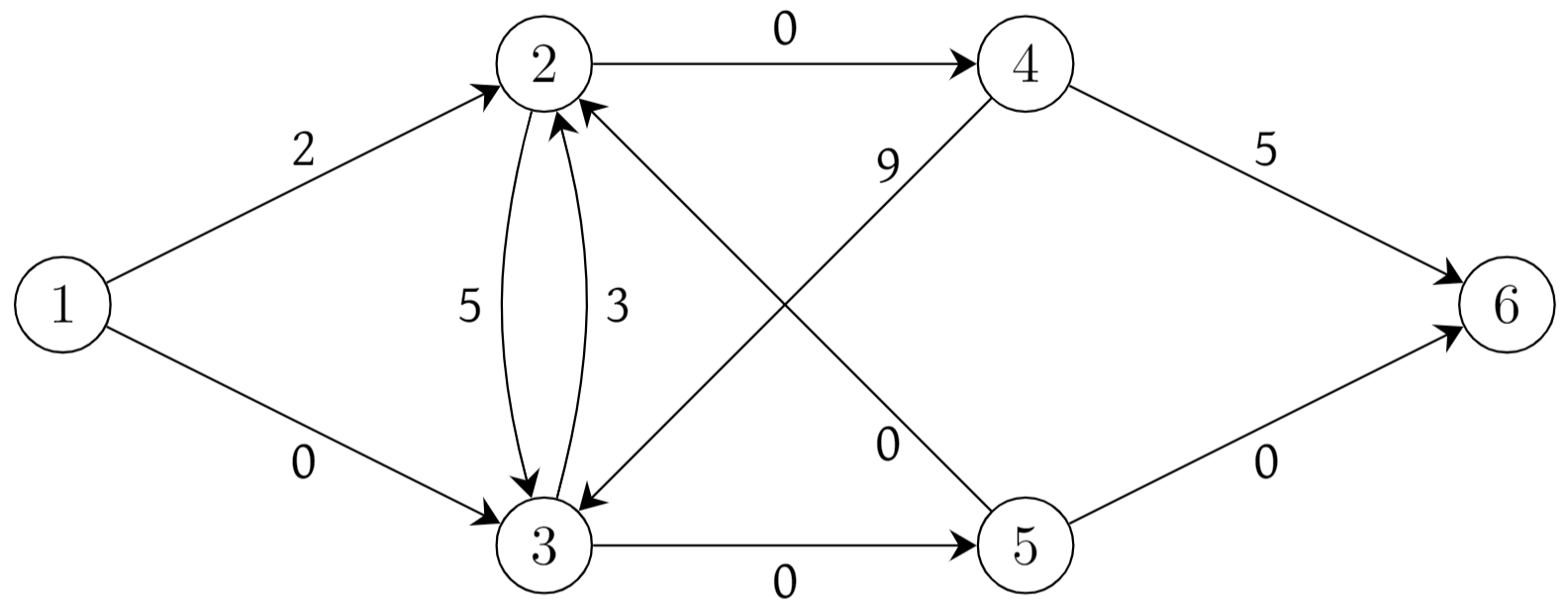
Fig. 2.8 Adjusted arc lengths

But what does this have to do with verifying that we got the correct answer for the shortest path from \(s\) to \(w\) in our original problem? First, let’s summarize what we just figured out. We give each node \(i\) a value \(p(i)\) (any value is possible). If we consider the problem where we try to find a shortest path from \(s\) to \(w\) with respect to the adjusted arc lengths \(\bar \ell(i,j) = \ell(i,j) +p(i)-p(j)\) (for each \((i,j) \in A\)) instead of the original ones \(\ell(i,j)\), then the shortest path found is also a shortest path for the original lengths. So we could solve the adjusted problem instead of the original one, if that turns out to be easier.

But how do we set the values \(p(i)\) for each node \(i \in N\)? Suppose we let \(p(i)=\) length of the shortest path from \(s\) to \(i\). (If we have run Dijkstra’s algorithm correctly, we presumably know these.) Do this for the graph in Figure 2.4; after all, we have already run Dijkstra’s algorithm for this graph, and the output from the algorithm gives us the proposed \(p\) value for each node. I claim that in computing the adjusted costs with these \(p\) values, you will rederive one of the figures given above. Which one is it? Do this exercise before continuing to read.

Next we will show that some of the properties of the adjusted lengths that you have just computed are not at all coincidental and hold when you perform this procedure for any graph whatsoever.

Claim 1. If, for each \(i \in N\), \(p(i)\) is set to the length of the shortest path from \(s\) to \(i\) (with respect to the original length function \(\ell\)), then, for each arc \((i,j) \in A\), \(\bar \ell (i,j) \ge 0\).

Proof. First observe that for each arc \((i,j) \in A\), the length of the shortest path from \(s\) to \(j\) is at most the length of the shortest path from \(s\) to \(i\) plus \(\ell(i,j)\) (since we can build a path from \(s\) to \(j\) by first going to \(i\) and then taking arc \((i,j)\)). By the way that we set the \(p\) values, this means that \(p(j) \le p(i) + \ell (i,j)\), and hence \( p(i) + \ell (i,j) -p(j) \ge 0\). Finally, \(\bar \ell (i,j) = p(i) + \ell (i,j) -p(j) \ge 0\).

Claim 2. If, for each \(i \in N\), \(p(i)\) is set to the length of the shortest path from \(s\) to \(i\) (with respect to the original length function \(\ell\)), then, for each node \(v \in N\), the total adjusted length of the shortest path from \(s\) to \(v\) is 0.

Proof. Recall that this shortest path is shortest with respect to both \(\ell\) and \(\bar \ell\). We know that the total adjusted length of any path from \(s\) to \(v\) is its total length with respect to the original lengths \( \ell\) plus \((p(s)-p(v))\). But \(p(s)=0\) and \(p(v)\) is the length of the shortest path from \(s\) to \(v\) (with respect to the original lengths \(\ell\)). So the total adjusted length of any shortest path is 0.

Claim 3. If, for each \(i \in N\), \(p(i)\) is set to the length of the shortest path from \(s\) to \(i\) (with respect to the original length function \(\ell\)), then, for each arc \((i,j)\) in a shortest path from \(s\) to \(v\), \(\bar \ell(i,j)=0\).

Proof. Claim 1 showed that each adjusted length is non-negative. Claim 2 showed that the total adjusted length of any shortest path is equal to 0. The only way these two can both happen is that every arc in a shortest path must have adjusted length equal to 0.

These claims have the following nice consequences. Suppose that you run Dijkstra’s algorithm. Now, if you compute \(\bar \ell\) where each \(p(i)\) is the shortest path length from \(s\) to \(i\), we get an equivalent input in which each arc has adjusted length that is non-negative, and each arc in a shortest path has adjusted length 0. Then by the simple special case that we discussed at the start (as in Figure 2.6), we know that we have the shortest path with respect to the adjusted lengths, and thus have the shortest path with respect to the original lengths.

Note

To summarize: we can check if our path from \(s\) to \(w\) is indeed shortest by

1. computing \(\bar \ell (i,j)\) for each arc in the graph for \(p\) values set by the shortest path lengths just found by Dijkstra’s algorithm;

2. for each \((i,j) \in A\), check that \(\bar \ell (i,j) \ge 0\);

3. for each arc \((i,j)\) in the path, check that \(\bar \ell (i,j) = 0\).

If this holds, then you have computed a correct shortest path.