Modeling with the Traveling Salesman Problem

1.3. Modeling with the Traveling Salesman Problem#

The traveling salesman problem is an important computational model for a variety of reasons. While the particular application of routing our poor salesman is valid enough, this does not really constitute a real-world application. However, it forms a central component of more complicated models, such as routing a fleet of vehicles for pickups and deliveries, or more concretely, the sort of problem that a UPS depot might solve on a daily basis. It can also be used to model a number of problems that, at first glance, do not seem to be related.

Of course, we have already encountered one such example. We can model the problem of determining the order in which the radio telescope observes the set of stars being studied as a traveling salesman problem. The set of stars to be studied corresponds to the set of cities to be visited. The re-positioning times \(\mbox{Focus-time}[i,j]\) correspond directly to the costs \(C[i,j]\). A feasible solution is again any permutation \(\pi\) of the stars, and the objective is to minimize the total re-positioning time for the telescope:

\[\sum_{i=1}^{n-1} \mbox{Focus-time}[\pi(i),\pi(i+1)] + \mbox{Focus-time}[\pi(n),\pi(1)].\]

It is important to note that this exactly captures what is needed in a 24-hour cycle of stellar observations. Hence, we could take our data for re-positioning the telescope, apply a standard software package for the traveling salesman problem (such as Concorde, which is the state of the art in this case), and be able to interpret the optimal solution for the corresponding traveling salesman input as an (optimal) solution to our telescope problem.

💡Demo

(Refresh page if not displaying.)

However, while modeling our telescope problem as a traveling salesman problem seems to make sense, and might work on some data sets, it also can fail miserably. Why?

There are both minor and major reasons why this model does not perfectly represent our computational problem. One notable minor issue is that our model of the problem views the telescope positioning problem as a perfect cyclical 24-hour problem. Recall that we had one week of access to the telescope to make observations. At the start of the week, we are taking over from how it was used the previous week by another astronomer. However, this is a minor discrepancy and would have only a small effect on the selection of a regular daily pattern.

There is a more fundamental issue that concerns the statement: a feasible solution is again any permutation \(\pi\) of the stars. That is not true for our problem. The telescope cannot be positioned to observe a particular star next if it is no longer above the horizon. Thus, to carefully and correctly model the telescope problem, we actually need a more complicated model that takes into account not just “travel times” and “waiting times” (while the telescope is observing a given star) but also so-called time-windows for each star that indicate the period of time (within each 24-hour cycle) that it is observable by our telescope as part of the input.

Even more generally, this suggests a good rule of thumb - when trying to model a problem in a decision-making setting, start by considering the simplest model! But before attempting to use that model to make actual decisions, it is important to test it to be sure that the “simplifying assumptions” made along the way are indeed the kind that can be put aside with minimal effect. Hence, the overall design process of thinking about a model might be viewed as follows:

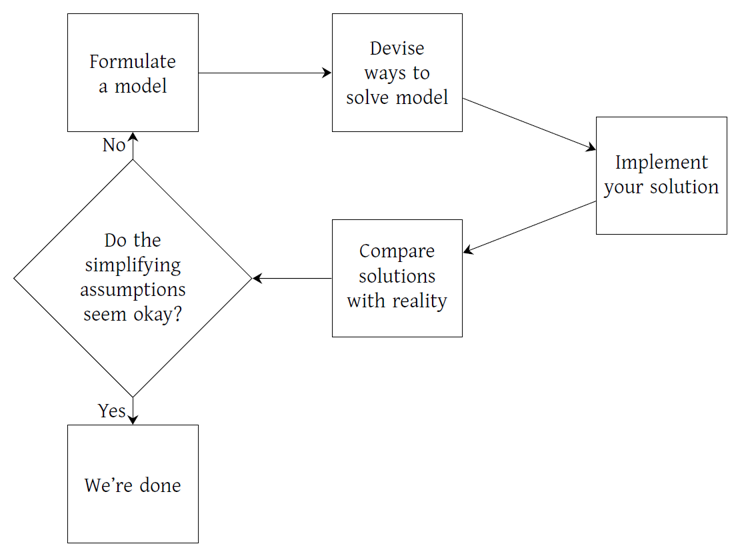
../../_images/process.png — Fig. 1.2 The cyclical process of formulating and analyzing an OR model#

Application: PCB Drilling#

In this part, we will consider a new problem to which the TSP can be applied: the manufacturing of printed circuit boards (PCBs). PCBs are used to mount integrated circuits and combine them with other hardware. Here is a picture of a PCB after the hardware has been mounted.

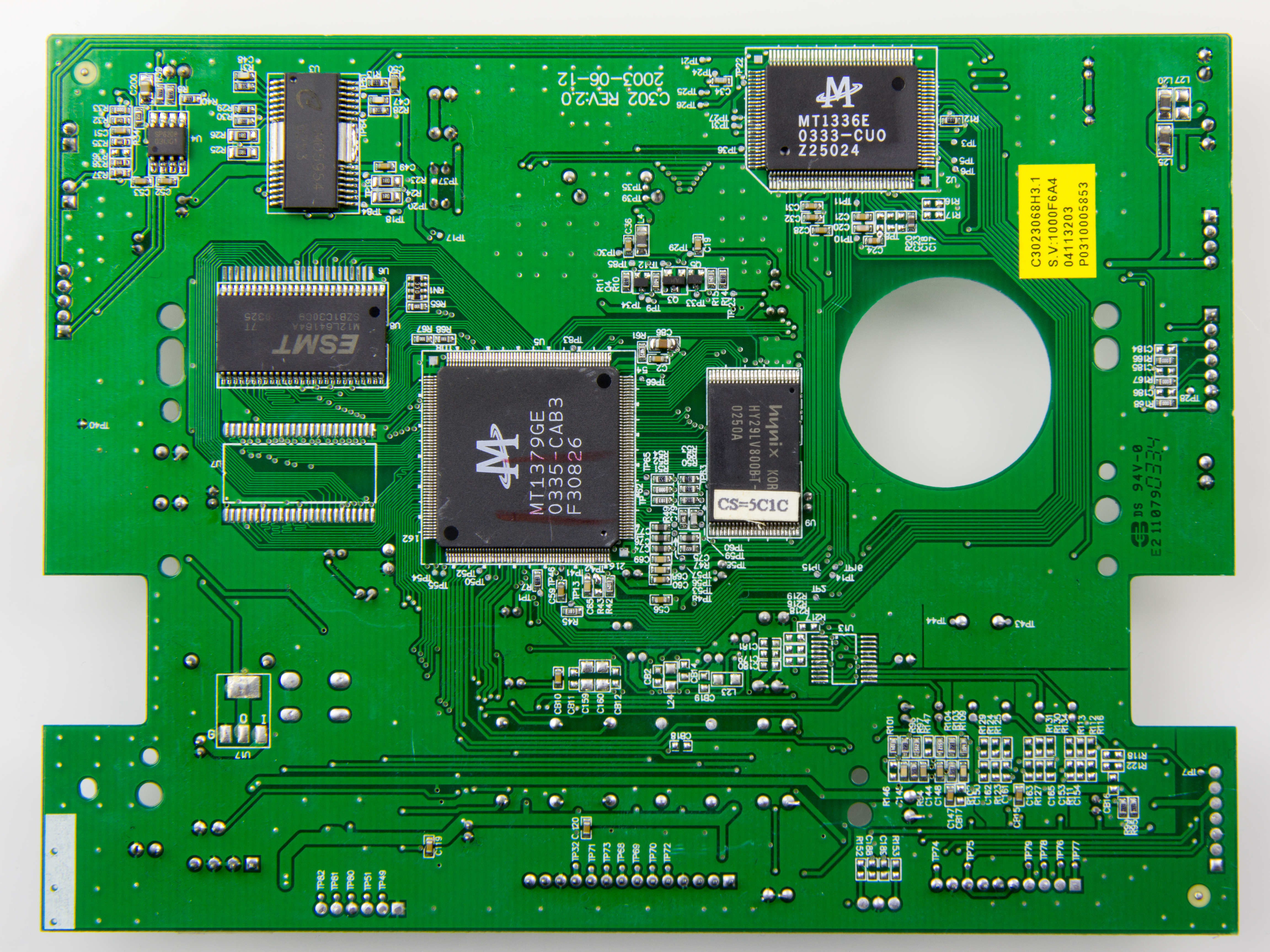
Taken from Wikipedia

Before the hardware can be mounted, a large number of small holes must be drilled in the board (see image below). The hardware is then mounted by placing the pins of the component in these holes.

Taken from AiPCBA

This sets up an optimization problem. Given a set of holes that must be drilled in a PCB, we must specify an order to drill these holes to our drilling machine. Our goal is to choose an order that minimizes the total distance the drill travels. Feeling déjà vu? This problem is analogous to the TSP!

Q: What are the “nodes” in the PCB drilling problem?

Q: What is the distance between two “nodes” in the PCB drilling problem? (Assume the drill can travel in a straight line from one hole to the next.)

Q: In answering the last two questions, you have fully described an input to the TSP. Assume we have a way of solving the TSP. How would you interpret the solution to the TSP (a tour of the nodes) as a solution to the PCB drilling problem?

Q: Why does the optimal TSP tour correspond to an optimal PCB drilling solution?

Let’s start by looking at a small PCB drilling instance: xqf131.

nodes = pd.read_csv('https://engri-1101.github.io/textbook/data/tsp/xqf131.csv', index_col=0)
nodes.head() # .head() restricts the display to just show the first 5 rows

# Like before, we need to construct a graph from this dataframe of nodes
G = vl.create_network(nodes)

Let’s apply some of our TSP heuristics and 2-OPT to get some good feasible solutions to this problem!

# Nearest neighbor
tour = vl.nearest_neighbor(G)
show(vl.tour_plot(G, tour))

# Improve with 2-OPT
show(vl.tsp_heuristic_plot(G, '2-OPT', tour=list(tour)))

# Nearest insertion
tour = vl.nearest_insertion(G)
show(vl.tour_plot(G, tour))

# Optimal
tour = optimal_tour('xqf131')
show(vl.tour_plot(G, tour))

Q: What were the following tour costs: nearest neighbor, nearest neighbor + 2-OPT, nearest insertion, and optimal? Which heuristic was closest to the optimal?

Next, let’s look at a well-cited PCB instance in TSP literature: pcb442.

nodes = pd.read_csv('https://engri-1101.github.io/textbook/data/tsp/pcb442.csv', index_col=0)
G = vl.create_network(nodes)

# Furthest insertion
tour = vl.furthest_insertion(G)
show(vl.tour_plot(G, tour))

# Optimal
tour = optimal_tour('pcb442')
show(vl.tour_plot(G, tour))

To make this problem more realistic, there is an added complication. We ignored where the drill bit starts and ends; it has to be the same location, usually in the corner. It is no longer good enough to just provide a tour of the holes to be drilled.

Q: If we just consider a tour of the holes, we miss two distances that must be traveled. What are they?

Let’s assume the start position of the drill is in the bottom left at \((0,0)\) and all of the holes to be drilled are at positions \((x,y)\) for \(x,y > 0\).

Q: How can we adjust our TSP input to account for this? (Hint: How does the set of nodes change, and what are the distances between them?)

If you look back at pcb442, you can see that the bottom-left node actually represents the drill start location and not a hole that needs to be drilled!

Modeling with the Traveling Salesman Problem

Contents

1.3. Modeling with the Traveling Salesman Problem#

Application: PCB Drilling#