Etching VLSI Computer Chips

1.4. Etching VLSI Computer Chips#

Now we want to show that sometimes problems that are not quite the same can still be modeled as TSP, in that we can use Concorde (or any other general purpose solver for this problem) to find an optimal solution. Here is such an example which arises in the process of manufacturing VLSI computer chips (VLSI stands for “very large-scale integration”, referring to the huge number of transistors that are integrated on a single chip). One step of this process can be viewed in the following simplified way: there is a square (a silicon wafer) on which one is going to etch a sequence of lines (electrical connections between different components of the chip). The machine doing the etching first moves to the correct position where the line starts and etches the particular line (as specified by the design) leaving it at a different point in the square. Then it must move to the correct position for the next line, and so forth. The lines may be etched in any order, but for each line, the etching must proceed in the specified direction (from the given starting point to the given ending point). The etching machine must start and end at the upper left-hand corner of the square (so as not to interfere with the square being put into and out of position for the etching). The VLSI etching optimization problem is to select an order for the lines to be etched so that as little time as possible is taken.

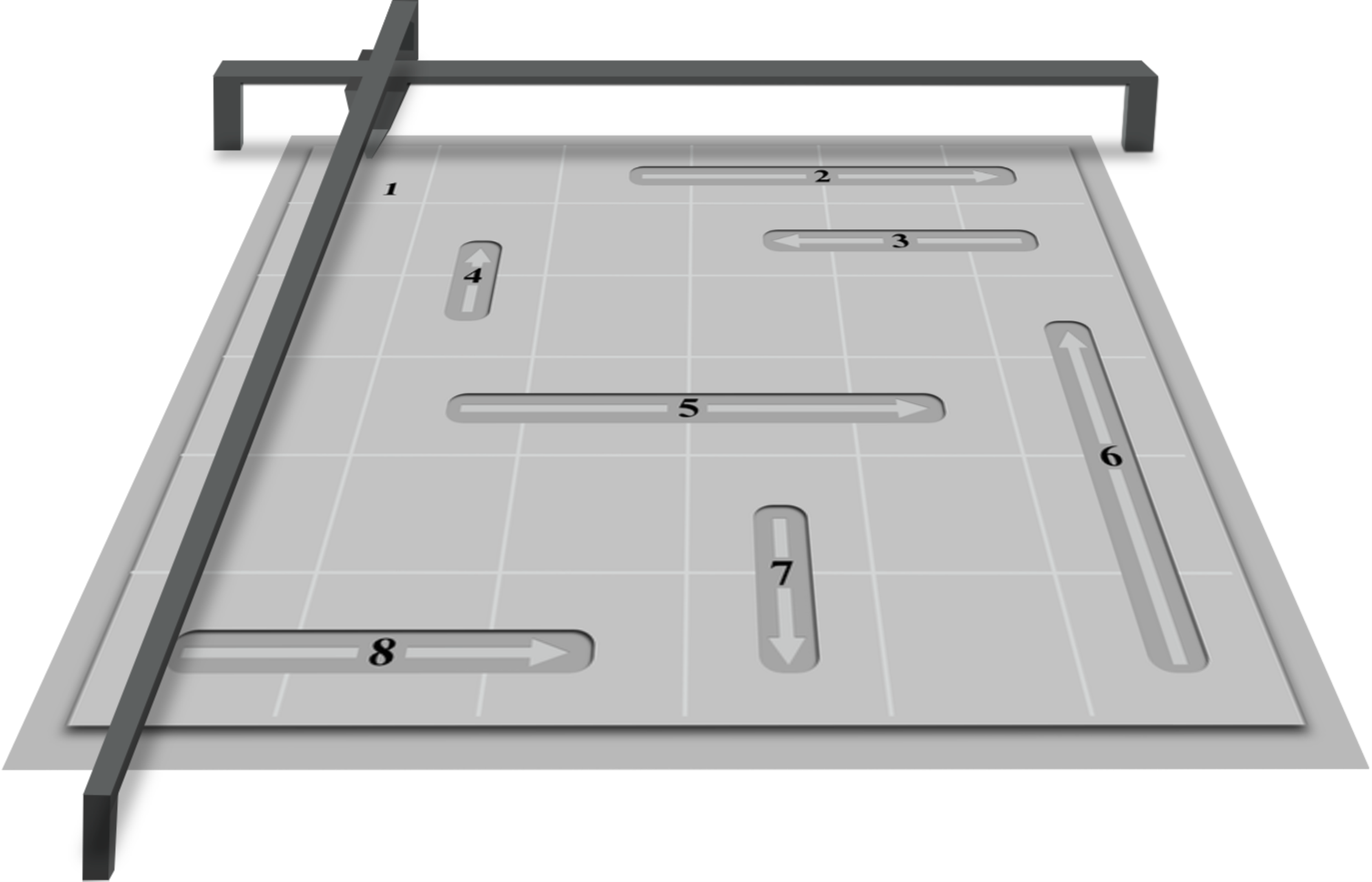
../../_images/etching.png — Fig. 1.3 A visualization of the VLSI etching optimization problem#

Q: What are the “nodes” in the VLSI etching problem?

Q: What is the distance between two “nodes” in the VLSI etching problem? (Assume the drill can travel in a straight line between two locations.)

We will show that this problem can be viewed as a special case of the traveling salesman problem, or in other words, can be modeled as one. More precisely, we will show that given any input to the VLSI problem, we can construct an input for the traveling salesman problem with the property that an optimal solution for this new input (that is, the cheapest tour) can be interpreted as an optimal solution for the VLSI problem. Suppose that \(N\) is a variable for the VLSI problem that specifies the number of lines in the input. From any given input to the VLSI problem with \(N\) lines, we will construct a TSP input with \(n=N+1\) cities; city 1 corresponds to the upper left-hand corner of this chip (at which the machine starts and ends its etching), and each of cities 2 through \(N+1\) corresponds to one of the \(N\) lines in the VLSI input.

The next observation is that in performing the etching of the lines, the machine’s time can be divided into two parts: the time actually etching the lines and the time moving the machine between lines when it is not actually etching. No matter what order in which the lines are etched, the time for the first part is the same. So, to minimize the total time for the machine, we should just minimize the total time that we are moving the machine without etching. If cities \(i\) and \(j\) both correspond to lines (so not special city 1) and the line corresponding to \(j\) is etched immediately after the line corresponding \(i\), then we spend the amount of time that it takes to move the machine from the endpoint of \(i\)’s line to the starting point of \(j\)’s line (while not etching). Furthermore, at the start, we move the machine from the upper left-hand corner to the starting point of the first line etched (while not etching). Finally, we move the machine from the ending point of the last line etched to the upper left-hand corner (while not etching). All of the periods in which the machine is not etching are considered in one of these cases. This motivates us to define the cost array as follows: let \(C[i,j]\) be the time to move the machine from the ending point of \(i\)’s line to the starting point of \(j\)’s line, for each \(i=2,\ldots,N+1,\ j=2,\ldots,N+1\); let \(C[1,j]\) be the time to move the machine from the upper left-hand corner to the starting point of \(j\)’s line, for each \(j=2,\ldots,N+1\); and let \(C[i,1]\) be the time to move the machine from the ending point of \(i\)’s line to the upper left-hand corner, for each \(i=2,\ldots,N+1\).

Q: Our past TSP examples have been symmetric in that the distance from node \(i\) to node \(j\) was the same as the distance from node \(j\) to node \(i\). Is the TSP input for a VLSI etching problem symmetric? Why or why not?

As we discussed previously, \(\pi\) can be specified so that the tour starts at any particular city, and therefore, we shall assume that \(\pi(1)\) is the special city \(1\). Our explanation above has shown that the total cost of any tour \(\pi\) is exactly the total time that the machine moves while not etching if the lines are etched in the order corresponding to \(\pi (2),\pi (3), \ldots, \pi(N+1)\). Consequently, if we find the best tour for the input \(C[i,j]\), \(i=1\ldots,N+1\), \(j=1,\ldots,N+1\), then this yields the ordering of the lines for which the total time to etch the chip is minimized.

Below, we have an example of a VLSI instance. The bottom-left node represents the starting location for the etching machine. Each line to etch has a blue starting point and a red ending point.

nodes = pd.read_csv('https://engri-1101.github.io/textbook/data/tsp/xqf131_etching.csv', index_col=0)
G = vl.create_network(nodes, directed=True, manhattan=False, x_i='x_start', y_i='y_start', x_j='x_end', y_j='y_end')
show(etching_tour_plot(G, [], width=600))

Again, we found we can use the TSP to solve this problem! Let’s start by applying some of our TSP heuristics. When printing the solution, the dashed lines indicate when the machine is moving between etchings.

# Nearest neighbor
show(etching_tour_plot(G, vl.nearest_neighbor(G), width=600))

# Nearest insertion
show(etching_tour_plot(G, vl.nearest_insertion(G), width=600))

# Furthest insertion
show(etching_tour_plot(G, vl.furthest_insertion(G, initial_tour=[0,70,0]), width=600))

Let’s see how these solutions compare to the optimal tour.

# Optimal
show(etching_tour_plot(G, optimal_tour('xqf131_etching'), width=600))

Q: Compare the heuristics’ performances. How did they compare to the optimal solution?

You may have noticed that we did not use 2-OPT to try and improve the tours. In fact, 2-OPT only applies when the distances are symmetric.

Bonus: Why does 2-OPT only apply when the distances are symmetric?

This completes the explanation that the VLSI etching problem can be modeled by the traveling salesman problem. Why was this an interesting thing to do? The traveling salesman problem is an extremely well-studied problem. Thousands of man-hours have been invested into devising software packages that solve the traveling salesman problem. By modeling the new problem, the VLSI etching problem, as a traveling salesman problem, we can build off of that experience and just solve our inputs for the etching problem by using the best software for the traveling salesman problem that we can find. This is one of the main reasons why it is beneficial to identify important models, including the next few topics, in the first place so that we can then use our experience in solving these models to solve other problems as well.